[DLAI 2018] Team 2: Autoencoder
This project is focused in autoencoders and their application for denoising and inpainting of noisey images. Furthermore, it was investigated how these autoencoders can be used as generative models, so-called Variational Autoencoders (VAEs). It was conducted in the context of the course Deep Learning for Artificial Intelligence at UPC (Autumn 2018) by the students Michaela Jurková, Michał Krzemiński, Michal Šimek and Daniel Seifert.
Motivation:
As none of us worked on Deep Learning before, we chose to start off with the rather simple topic of autoencoders in order to learn how to built a neural network, how to train it and how the setting of hyperparameters affect its performance. Moreover, we found interest in autoencoders due to their versatile applications in pattern recognition and classification, denoising and even in generation of completely new data.
Goals:
Step 1: Implementation of a simple autoencoder in Keras:
- Learn how autoencoders work
- Build first examples based on the tutorials based on i.a. the MNIST data set
- Investigate performance changes for varying parameters
Step 2: Implementation of a denoising and inpainting autoencoder:
- Preprocess picture data set by adding noise manually
- Make hyperparameter adjustments to improve its performance
- Apply the denoising and inpainting to more complex datasets
Step 3: Implementation of Variational Autoencoder (VAE)
- Learn how VAEs work using the MNIST data set
- Investigate performance changes when extending the latent space
- Apply it to more complex datasets
What is an autoencoder
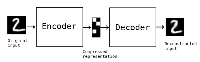
Autoencoder refers to a artificial neural network where the input data are compressed by an encoder and this compressed representation is then fed into a decoder to be decompressed into the reconstructed output which is lossy. It is learned automatically from data examples. Because autoencoders are data-specific, they can only be used with applications using data similar with the data the particular autoencoder have been trained on and won’t really work with different data.
Denoising autoencoder with MNIST dataset
Preparing the data
We loaded the MNIST images without the labels because we don’t need them. After that, we normalized the loaded data values into 0-1 of 32-bit float data type and then reshaped it to the array suitable for the network.
Model of autoencoder
For the encoder, we used a stack of two Conv2D (2D convolution layer) and MaxPooling2D (2D pooling layer) layers. RelU activation function was used with both Conv2D layers. For the decoder, we used the stack of two Conv2D with RelU activation and MaxPooling2D layers again, followed by the last layer of a Conv2D with Sigmoid activation function. We used the convolutional neural networks because on images they perform much better than the other types. We set the AdaDelta optimizer and Binary Cross-entropy loss function for our model.
Creating a corrupted images
We created a synthetic corrupted images as an input images for our denoising and inpainting autoencoder. We created a three types of images corruption: applied a noise, generated a randomly placed horizontal black stripes (10 stripes over 28 rows) and created a randomly placed gray block of size 10x10 over the original images.
Training the network
We trained the network for 100 epochs with batch size of 128. We used the corrupted images as an input of the autoencoder and the original images as a desired output in order to train the autoencoder to map the corrupted input images into the clean output images. After training of the 100 epochs, we got the losses values slightly less than 0.1.
Results
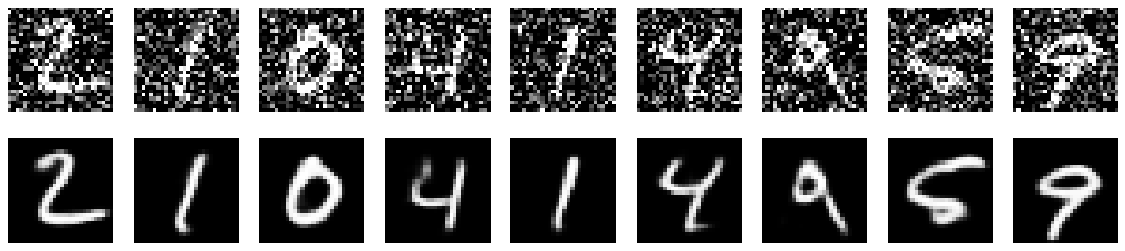
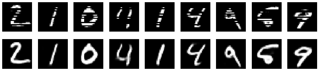
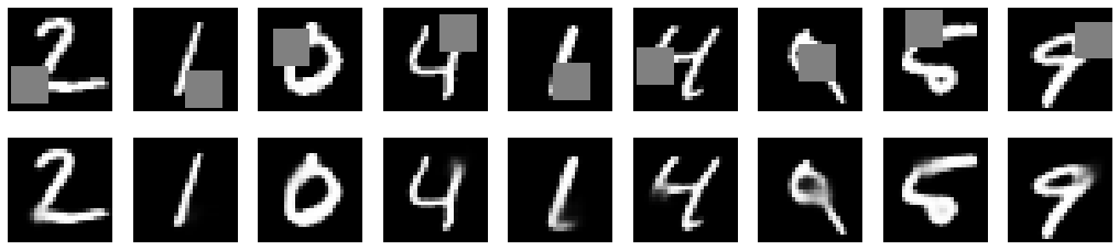
In the following pictures are shown the results of our trained autoencoder on MNIST digits. The first line corresponds to the input corrupted images and the second line corresponds to the reconstructed output.
Noisy images
Images with stripes
Images with gray blocks
Denoising autoencoder with anime characters images
After applying denoising and inpainting on the MNIST images, we tried to implement the denoising and inpainting tasks using autoencoders on a real images to see how it will perform.
Used datased
We used the dataset accessible from this link. It consists of 14490 color images of an anime characters faces in total. The images have an uniform size of 160x160.
Preparing the data
As a first step, we split the dataset into a train (70%), validation (15%) and test (15%) parts. We used the OpenCV library for reading the images and resizing them into a size of 64x64 because it is sufficient for us and it significantly reduces the time needed for training the network. Because the library uses a BGR color space as default, we also converted the images into the RGB color space. Then we normalized the values into 0-1 and reshaped into the array suitable for the network just like in the MNIST denoising case.
Model of autoencoder
Input is 64x64 image with 3 color channels. An encoder consists of a pair of Conv2D (first has 64 filters, second has 32 filters) and MaxPooling2D layers again and a decoder consists of a pair Conv2D (first has 32 filters, second has 64 filters) and MaxPooling2D layers followed by the Conv2D layer again. The optimizer and the loss function is also the same as in the MNIST case.
Creating a corrupted images
We created corrupted images from the original images in the same way as in the MNIST case. We used noise factor 0.3 for gaussian noise, 24 horizontal black stripes for images with stripes and gray blocks of size 24x24 for images with blocks.
Training the network
The training was the same as in the MNIST case. After 100 epochs, we got the losses values around 0.49.
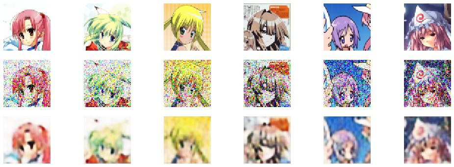
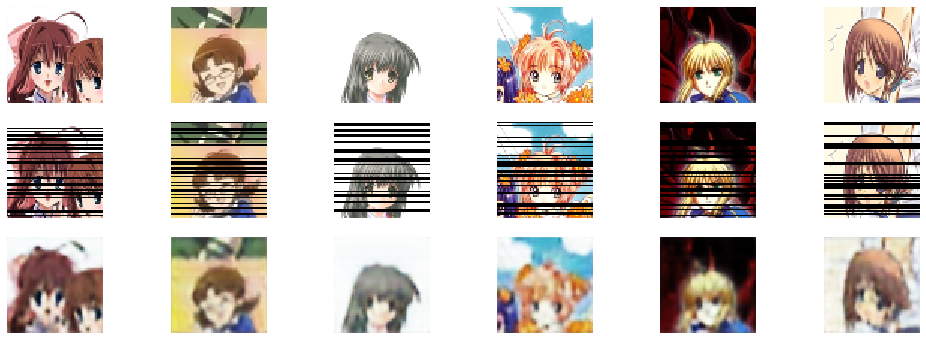
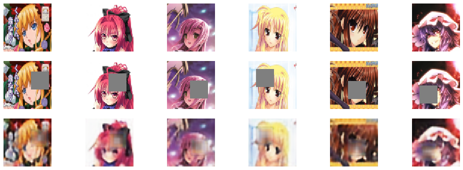
Results
In the following pictures are displayed the results of our trained autoencoder on MNIST digits for the noisy images, images with stripes or images with gray blocks in the input. The first line corresponds to the original image before we corrupted it, the second correspond to the input corrupted images and the third line corresponds to the reconstructed output.
Noisy images
Images with stripes
Images with gray blocks
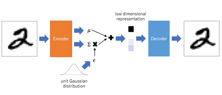
Variational Autoencoder (VAE)
In order to transform our autoencoder into a generative model some adjustments have to be made:
- The latent space has to be restricted to follow a defined probability density functions such as a Gaussian distribution. In the end we want to generate new data from a previously trained autoencoder by sampling from this latent space.
- This moreover creates another problem for us: Since we want to train our network using gradient descent and backpropagation cannot flow through random nodes, we have to apply the so-called reparameterization trick. Instead of sampling from the distribution at the end of the encoder, we sample from an ε, that is normally distributed and further on multiplied to the variance of our encoder distribution. Thus, the random node is “outsourced” and gradient descent can be calculated without any problems.
- We extend our loss function (the reconstruction loss) with an additional regularization term, the Kullback-Leibler (KL) divergence, which measures the difference between the distribution (in the encoder), that projects our data into the latent space, and our true latent probability distribution (Kristiadi: Variational Autoencoder: Intuition and Implementation).
VAE for the MNIST dataset
As for the denoising autoencoder we start to train it first with the standard MNIST dataset in order to understand how the VAE essentially works. We keep the same structure that is composed of multiple convolutional and pooling layers, and apply the changes mentioned in the paragraph above, that adds the reparameterization trick in the bottleneck and the KL divergence term to our loss function.
After the neural network has been training for 100 epochs and a batch size of 128, we can randomly generate noise and sample from the decoder part of our network to obtain new digits:

For a neural network as ours with a two-dimensional bottleneck, the distribution of the generated digits in the latent space can be easily visualized as follows:


VAE for the Anime dataset
After testing the VAE with the standard MNIST dataset, we move on to investigate its performance again on a more complex dataset, the Anime dataset. The structure of our VAE stays the same, but we experiment now with the dimensionality of our latent variable space.
Dimensions in latent space = 2

Dimensions in latent space = 5

Dimensions in latent space = 100

Discussion
It can be clearly seen that the features in the newly generated images increase with higher dimensionality in our latent space. The image itself is compressed less in the bottleneck and therefore, more detailed pictures can be generated out of this latent space. Another surprising aspect are colors of the generated images, that seem to vanish for lower dimensional sizes due to compression.
Future Work
To furthermore investigate the behavior of variational autencoders and strengthen their performance, the simple Gaussian distribution can be mapped to more complex distributions in order to achieve even better results. This method is called Normalizing Flows.