Neural Style Transfer
Project carried out by ETSETB students as part of the Deep Learning for Artificial Intelligence subject. This notebook contains the research and discussion performed of the state-of-the-art NST techniques.
Results obtained
This document has been generated to explain the different results that have been obtained from the Neural Style Transfer repository. All the results have been developed using the Google Cloud platform. A Virtual Machine with 16Gb of RAM and an specific GPU helped in executing all the algorithm iterations. The document will be scheduled as it is shown below:
- Google Cloud Environment
- Results Generation
- Results Comparison
- Init variables
- Results of iterations
- Results analysis
- Tuning Content weight and Style weight
- Total variation weight
- Style Layers
- Content Layers
- Image Size
- Initialization
Google Cloud Environment
The following requirements have been installed in a VM on Google Cloud:
- Tensorflow
- Keras
- CUDA (GPU)
- CUDNN (GPU)
- Scipy + PIL
- Numpy
- h5py
All the requirements have been installed in a virtual environment with the main repository cloned in it. In the Neural-Style-Transfer folder, a new directory have been declared to save the results of the execution for each iteration.
Results generation
The main execution code called Network.py has been modified in order to save and manage the information of each iteration. This new Python file called Network_modified.py store the values of loss, time and improved performance in three independent vectors. At the end of all iterations, this vectors contain the data that is saved in three different graph plots.
Furthermore, to have a reliable reference of the NST performance, the first 10 iterations are saved (where the improvement is higher) and later on only the multiples of 10. At the end, we obtain a final output directory with 19 images of the style transfer evolution, three more images that contain the data stored (time, loss function value and improvement) and a .txt file with all the parameters used.
To speed up the process of generating different outputs for each parameter changed, two scripts have been declared. The first one compress the /outputs/ directory to be downloaded, the second one cleans all the directories and prepare the repository to perform another simulation.
Results comparison
The Neural-Style-Transfer repository have a default configuration of values such as convolutional layers, style weight, content weight or init variables. In the following table all the default parameters are shown.
| Parameter | Default Value | Possible values |
|---|---|---|
| –num_iter | 100 | 200 |
| –content_weight | 0.25 | 0.25 - 1 - 100 - 1 |
| –style_weight | 1 | 1 - 0.25 - 1 - 100 |
| –tv_weight | 8.5e-5 | 1e-4, 1e-5, 1e-8, 5e-8,1e-20 |
| –img_size | 224 x 224 | 224x224- 112x112 - 448 x 448 |
| –content_loss_type | 0 | 0 - 1 - 2 |
| –content_layer | conv5_2 | conv1_1 - conv1_2 - conv2_1 - conv2_2 - conv3_1 - conv3_2 - conv3_3 - conv4_1 - conv4_2 - conv4_3 - conv4_4 - conv5_1 - conv5_2 - conv5_3 - conv5_4 |
| –pool_type | max | max - ave |
| –init_image | noise | content - noise - gray |
All of this parameters, with the exeption of –content_layer, that has to be modified directly in the code, are set in the initial command when the execution is performed. To have a clear reference of how the Neural Style Transfer is working, 36 different experiments have been proposed.
The following table contain all the tests made with an identifier. All of this experiments can be found in /2018-dlai-team5/Results/ in which the name of the folder is the identifier of the table.
| Test number | Modified parameter with respect to default | Test number | Modified parameter with respect to default | |
|---|---|---|---|---|
| 1 | Default configuration | 18 | [‘conv1_1’, ‘conv3_1’, ‘conv5_1’] | |
| 2 | style_weight = 0.25, content_weight = 1 | 19 | [‘conv1_1’, ‘conv3_1’] | |
| 3 | style_weight = 100, content_weight = 1 | 20 | Cristian face | |
| 4 | style_weight = 1, content_weight = 100 | 21 | Clara face | |
| 5 | tv_weight = 1e-4 | 22 | Guillem face | |
| 6 | tv_weight = 5e-4 | 23 | Marc face | |
| 7 | tv_weight = 1e-8 | 24 | pool_type = ave | |
| 8 | tv_weight = 1e-20 | 25 | init_image = gray | |
| 9 | [‘conv1_1’, ‘conv2_1’, ‘conv3_1’, ‘conv4_1’, ‘conv5_1’] | 26 | [‘conv1_1’, ‘conv2_1’] | |
| 10 | [‘conv1_1’, ‘conv2_1’, ‘conv3_1’, ‘conv4_1’] | 27 | Cristian init_image=content | |
| 11 | [‘conv1_1’, ‘conv2_1’, ‘conv3_1’’] | 28 | Image size 112 | |
| 12 | [‘conv1_1’, ‘conv2_1’] | 29 | Image size 448 | |
| 13 | [‘conv1_1’] | 30 | Conv layer 1_2 | |
| 14 | [ ‘conv2_1’, ‘conv3_1’, ‘conv4_1’, ‘conv5_1’] | 31 | Conv layer 2_2 | |
| 15 | [‘conv3_1’, ‘conv4_1’, ‘conv5_1’] | 32 | Conv layer 3_2 | |
| 16 | [ ‘conv4_1’, ‘conv5_1’] | 33 | Conv layer 5_2 | |
| 17 | [‘conv5_1’] | 34 | Conv layer 5_2 content_weight = 100 style_weight = 1 |
To execute the different tests, two images have been selected as default.
- Content:

This content image selected for the different textures (grass, leaves,fur,grille), objects( dog, floor, hose, background) and colors in the image.
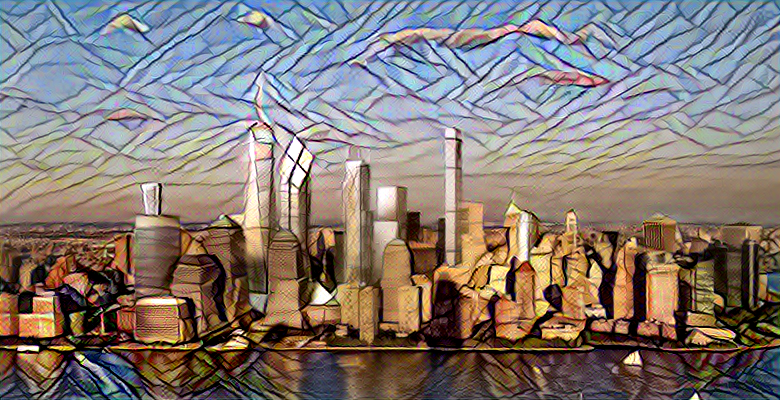
- Style:

This image was selected because is one of the most typical in datasets of transfer stlyle. The image has a very particular texture and colors, and some elements (like the building and the moon) that are quite characteristic.
Results of iterations
As it has been introduced before, in each experiment the Neural Style Transfer code gives us an output image accordint to each iteration. Our modified code provide us he first 10 images according to their iterations and later on the corresponding 9 ones in steps of 10. The following image is an example of all output images in a default parameters iteration:

In the first image (that correspond to initial random image after one iteration) we can recognise some shapes. The follow iterations show more details about the textures, objects and define the primary colors. Iterations 20, 30 , 40 , 50, 60, 70, 80, 90. Iteration number 100 shows much better result if we compare it with the initial ones. The main reason is that atter iteration number 10, the loss function is converging, so is better analyze 1 photo of each 10 iterations. Now, each photo show little improves from the lasts iterations, but at the end this improvements are so small that we can presume that around the 50 iteration we get the final image, but we still calculating 100 in order to analyze different loss function for different hyperparameters.
Loss function:
The function converge around 20 iterations in almost all tests made with 224x224 image size. At image at 50 the resulting image is practically equal than image at 100.

In order to evaluate more accurately the improvement of the image iteration after iteration, this image show the percentile of reduction of function loss between iterations.
Improvement function

It is quite clear to see that in the first iterations the improvement value is very high. The value depends on the input variables initialization but specially in the image size. The bigger the image is, the more iterations are needed to converge, so the improvement value is distributed in a more homogeneus way on the first 20 iterations.
Time function:

The results in time function are quite correlated to the improvement function. The execution time for each iteration will increase drastically if we increase their size.
Results analysis
Because of the huge amount of images as a result of all the test made, we will add a reference of a Google Document with all labeled images to check the final observations. In the following list, we will present the different modifications made and the conclusions we have extracted.
Tuning Content weight and Style weight:
The relation between those parameters affects directly in the priority of the algorithm to keep the information of style image or content image. If content weigh is bigger than style weigh, the generated image will be more similar to content image and vice versa.
The relation of these parameters produce variations. Changing the parameters but keeping the proportion doesn’t produce any important modification.
(Figure 0)  Content weight =0.25 and  Style weight = 1
(Figure 1)  Content weight =1 and  Style weight = 0.25
When we invert the parameters of content weight and style weight, is easy to see some changes in the image. In the original configuration, the leaves (top left) and grille (top right) have a different texture than in the Figure 1, where the original texture is more recognizable. Texture of grass and the fur are similar in both images.
Despite that, colours are quite different. In Figure 0 is easy to see the influence of the color of Style image, some parts, originally the darkest surfaces, are colored in blue. In Figure 1, the original colors remain intact if we compare it with the previous one.
(Figure 2) Content weigh =100 and Style weight =1
In that case, the influence of style image is reduced at minimum. Original colors are keeped totally. The only change from the content image are changes in texture, some kind of blurred.
(Figure 4) Content weigh =1 and Style weight =100
Influence of style image is total. Still keeping some remainder from the leaves and the grill textures, but the grass has disapeared. Elements from the Style image are included without coherence with the content. It is easy to se how appear in the middle of the image an structure similar to the building of image style. Original colors have been totally lost.
Total variation weight:
(Figure 5) TV=0.0001
(Figure 6) TV=0.0005
(Figure 7) TV=8.5e-5
(Figure 8) TV=1e-08
(Figure 9) TV=1e-20

Total Variation Weight try to avoid blurred effect in image. Values closest to 0 increased this effect, so the final result has more quality but the execution time is higher. This value also affects in the color of the image. Values far from 0 on this parameter prevent the appearance of style image colors and values close to 0 helps to expand it.
Style Layers:
Probably this hyper parameter is one of the most interesting and difficult to text (for the high number of combinations). So, in order to analyze it in a reliable way, some of the most interesting configurations have been tested. The weight of each layer is configurated according to the number of layers, so the weight of style layers re.
(Figure 10)  ['conv1_1', 'conv2_1', 'conv3_1', 'conv4_1','conv5_1'] (original values)
(Figure 11)  ['conv1_1', 'conv2_1', 'conv3_1', 'conv4_1']
(Figure 12)  ['conv1_1', 'conv2_1', 'conv3_1']
(Figure 13)  ['conv1_1', 'conv2_1', 'conv3_1']
(Figure 14)  ['conv1_1']

As we can see in the previous results, deleting style layers starting from the deeper ones to the higher ones we can see how eventually the output image looks more similar to content image, starting with little changes in the color. The changes in the texture are little different in each image, loosing detail and beeing more general. The last image, where only conv1_1 is maintained, shows how the main changes made reside in colours, but keeping the original texture as well. The reason is that the first layers in the network are based in evaluating the pixels, so the high level features characteristics from the structure of style image are lost.
Comparing those two image above, it is easy to see how the foreleg and the snout are lees defined in Figure eight figure than in the left one, where conv5_1 can provide more high level details.
<img width="400height="300src=" https://github.com/telecombcn-dl/2018-dlai-team5/blob/master/Utils/two.png">
(Figure 15)  ['conv2_1', 'conv3_1', 'conv4_1', 'conv5_1']
(Figure 16)  ['conv3_1', 'conv4_1', 'conv5_1']
(Figure 17)  [ 'conv4_1', 'conv5_1']
(Figure 18)  ['conv5_1']

Without conf3_1, transfer style keep the color from the content image, texture is only different from the original for blurred effect. Looks like ‘conv1_1’,’conv2_1’ and ‘conv3_1’ have more influence in color than ‘conv4_1’ and ‘conv5_1’. That makes sense because are more closest to pixel value. Our intuition is that ‘conv4_1’ and ‘conv5_1’ are more focused in details, providing more defined textures in concrete elements of the image. Without a base to represent high level details, conv4_1 and conv5_1 are useless.
The next tests are related to groups of layers, selected to combine high level and down level features.
(Figure 19) ['conv5_1']
This example shows that keeping intermedial layers improve the realistic effect of the artistic style, providing better final results. Some effects are no coherent with the context of the image, merging the dog with the floor.
(Figure 20) ['conv1_1', 'conv5_1']
The effect of the layers from the extremes doesn’t change textures, only color and is quite similar to Figure 14, where only conv1_1 is used. Furthermore, in the following result we can see the high of detail in features. We can state that the final result is visually abrupted. In Figure 22 we can see how the texture applied is low level. Poorly detailed and has no coherence with the elements of the image
(Figure 21)  ['conv1_1', 'conv5_1']
(Figure 22)  ['conv1_1', 'conv5_1']
Content Layers:
Content layer affects on how measure content style in the final result. High level layers will provide high details, but small focus in pixel value. Low level layers will provide pixel fidelity, but less flexibility to style transfer. In the following experiments we can see the different values of content layers.
(Figure 23)  Content Layer = Conv1_2
(Figure 24)  Content Layer = Conv2_2
(Figure 25)  Content Layer = Conv3_2
(Figure 26)  Content Layer = Conv4_2 (default configuration)
(Figure 27)  Content Layer = Conv5_2
(Figure 28)  Content Layer = Conv5_2 Content_weight= 100 Style_weight= 1

Using Conv1_2, Conv2_2 and Conv3_2 as content layers, the most part of the original pixel values is maintained. The lower level the layer is, the bigger the similarity with content image we can see. Using this measures for content image is too restrictive to see a clear style transfer effect.
Conv5_2 layer loose drastically the result so it is imposible to recognise content image. This happens probably because the references are taken from a values to far from the original pixels. By changing the content and style weights is possible to reduce this effect.
Image Size:
Image size has a direct impact in the final results, especially when the size of the input content is reduced. VGG16 and VGG19 originally are prepared to work with 224 x 244 x 3 images, but this can be modified through the input variables. So, optimized results are for this size of image.
(Figure 29)  Image size = 224 x 224 (original configuration)
(Figure 30)  Image size = 112 x 112
(Figure 31)  Image size = 448 x 448
Increasing the size of the image taking into account the reference of 224 the final result look quite similar, but more high defined due to the information provided. If we reduce the size, the resulting image have more noise effects, is difficult to recognise content and colors and texture are included without sence from the original content. The execution time is higher if the image size is increased.
Initialization:
Usually, style transfer start drawing from random image, but can also work over content image. That reduces the noise effect in the output image and the final result is much better. Starting from the content, we cna see that has a direct impact in the way how style image is applied. In that case, style image only affects one part of the image, producing color and texture variations. But the rest of the image remains intact. This is because loss function converge with these changes, and do not obtain any improve changing the rest. To achieve a better result, it is necessary to modify Style and Content weight.
(Figure 29)  Initialization = Gray
(Figure 30)  Initialization = Content
The rest of the results can be checked in the directory. Each experiment has the first 10 images of all iterations and multiples of 10 to the end. In each experiment, loss, time and execution improvement functions can be check as well as the .txt file that contains all the simulation parameters. Because of the limited execution time in Google Cloud, the last 8 tests do not contain the plots of this functions because the execution was performed using Colab. Despite this, the final output image at iteration number 100 is preserved to analyze the final impact of the variables changed.